
Build mini TensorFlow-like library from scratch
If you are really curious about the state of the art of machine learning, then you know the guts of crashing down a computationally hard problem from scratch. and, You might have noticed what libraries like Tensorflow, Pytorch, or Keras are capable of.
In this blog post, I will try to break down some fundamentals of differentiable graphs which is a building block of the TensorFlow library. we will build a small library to train and test an artificial deep neural network from scratch.
Since we are generally dealing with Artificial neural networks here, I assume it’s not your first time hearing about it. If I am wrong then, worry not. I wrote something for you back then when-i-use-a-word-artificial-intelligence. But basically, ANNs mimic the process of how our (human ) brains operate, and it's a biologically inspired computational network. sounds pretty scary right?
Computational wise you might have to think of it as a graph of mathematical functions such as linear combination and activation functions. The graph consists of nodes, and edges. Just like this image down.

Nodes in each layer perform mathematical functions using inputs from nodes in the previous layers or input predictors (for nodes in the input layer). For example, a node could represent simple linear function f(x,y)=x+y+b, where x and y are input values from nodes in the previous layer or simply inputs(for nodes in the input layer), and b is a bias unit.
Each node creates an output value that may be passed to nodes in the next layer or if the node is in the output layer then it produces a target variable. The Layers between the input layer and the output layer are called hidden layers.
The edges in the graph connect the nodes where the values flow from one layer to the other. These edges can also apply operations to the values that flow with them, such as multiplying by weights and adding biases.
Considering how we can implement graph structure in our mini Tensorflow_like library, We’ll use a Python class to represent a generic node. each node might receive input from multiple other nodes (inbound_nodes). each node also creates a single output, which will likely be passed to other nodes (outbound_nodes).
by adding two lists (one to store references to the inbound nodes, and the other to store references to the outbound nodes), each node will eventually calculate a value that represents its output. the code snippet below shows the implementation in python.
class Node(object):
    def __init__(self, inbound_nodes=[]):
        # Node(s) from which this Node receives values during forward pass.
        self.inbound_nodes = inbound_nodes
        # Node(s) to which this Node passes values during forward pass.
        self.outbound_nodes = []
        # For each inbound_node, we add the current Node as an outbound_node as it is.
        for n in self.inbound_nodes:
            n.outbound_nodes.append(self)
        # A calculated value initiated to none
        self.value = None

        # Forward propagation (forward pass)
        def forward(self):
        """
        Compute the output value based on `inbound_nodes` and
        store the result in self.value.
        """
        raise NotImplemented
Unlike other hidden layers nodes, the Input nodes subclass doesn’t have inbound nodes as they are the frontier of our neural network .they do not actually calculate anything. They hold a value, such as a data feature or a model parameter (weight/bias). value can be set either explicitly or with the forward() method, and This value is then fed through the rest of the neural network during Forward propagation.
below is the implementation of the input node.
class Input_node(Node):
    def __init__(self):
        # An Input node has no inbound nodes,so no need to pass anything to the Node instantiator.
        Node.__init__(self)

    def forward(self, value=None):
        # Overwrite the value if one is passed in.
        if value is not None:
            self.value = value
Forward Propagation
By propagating values from the first layer (the input layer) through all the mathematical functions represented by each node(the nodes of the hidden layer), the network outputs a value. This process is called a forward pass.
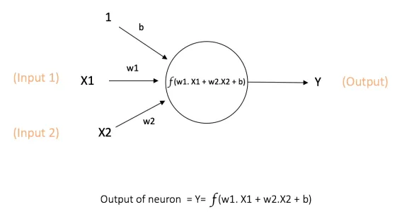
The picture above shows just a simple perceptron with two inputs and a bias unit to produce the output after performing a mathematical function, with no hidden layers.
Let’s implement a forward pass with two methods to help us define and then run values through our graphs, we will Implement the topological_sort method and forward_pass. Given the fact that the input to some nodes depends on the outputs of others, we need to flatten the graph in a way where all the input dependencies for each node are resolved before running its calculation. we will use topological sort.
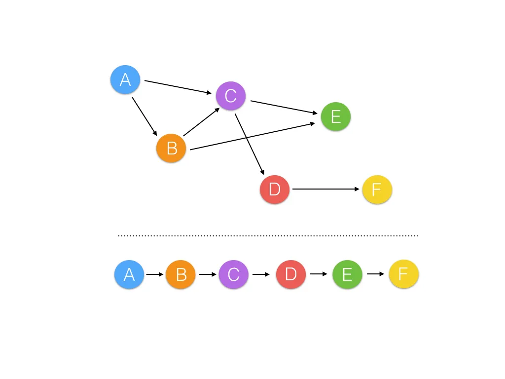
it is just a Depth-first search algorithm where we take one node and expand to its end roots before continuing to the next one. It only works with Directed_acyclic_graphs. the animation below explains a depth-first search algorithm in details
The topological sort function will return a sorted list of nodes in which all of the calculations can run in series. takes in a feed_dict, which is a dictionary data structure where we initially set a value for an input_node. Here's the code implementation.
def topological_sort(feed_dict):
    """
    Sort generic nodes in topological order using Kahn's Algorithm.

    `feed_dict`: A dictionary where the key is a `Input` node and the value is the respective value feed to that node.

    Returns a list of sorted nodes.
    """

    input_nodes = [n for n in feed_dict.keys()]

    G = {}
    nodes = [n for n in input_nodes]
    while len(nodes) > 0:
        n = nodes.pop(0)
        if n not in G:
            G[n] = {'in': set(), 'out': set()}
        for m in n.outbound_nodes:
            if m not in G:
                G[m] = {'in': set(), 'out': set()}
            G[n]['out'].add(m)
            G[m]['in'].add(n)
            nodes.append(m)

    L = []
    S = set(input_nodes)
    while len(S) > 0:
        n = S.pop()

        if isinstance(n, Input):
            n.value = feed_dict[n]

        L.append(n)
        for m in n.outbound_nodes:
            G[n]['out'].remove(m)
            G[m]['in'].remove(n)
            # if no other incoming edges add to S
            if len(G[m]['in']) == 0:
                S.add(m)
    return L
We have to have a way to run the network and output the value, The method forward_pass() down here will perform that for us.
def forward_pass(output_node, sorted_nodes):
    """
    Performs a forward pass through a list of sorted nodes.
    Arguments:
        `output_node`: A node in the graph, should be the output node (have no outgoing edges).
        `sorted_nodes`: A topologically sorted list of nodes.
    Returns the output Node's value
    """

    for n in sorted_nodes:
        n.forward()

    return output_node.value
Time for big hows!
How do we turn our neural network into a learning machine(human-like) then?
The first step lets make our neurons (nodes ) linear
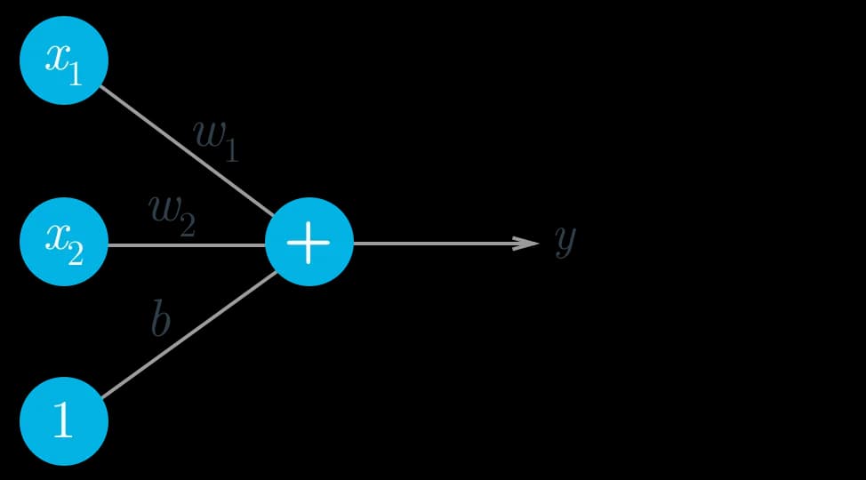
As I stated back on top, we should think of ANN as “a graph of mathematical functions such as linear combination and activation functions. The graph consists of nodes, and edges”. now think of node as a neuron or linear function with an activation function wich is addition operator in the image down here. and think of edge as simply three main components of linear fumction (weights wi, inputs xi, and bias b) . so our neuron is just the weighted sum of the inputs plus the bias for now.
Under this linear node(neuron ) our network is finally becoming a clear thinker(smart is overrated). here is an implementation of a simple linear node.
class Linear(Node):
    def __init__(self, inputs, weights, bias):
        Node.__init__(self, [inputs, weights, bias])

        # NOTE: The weights and bias properties here are not
        # numbers, but rather references to other nodes.
        # The weight and bias values are stored within the
        # respective nodes.

    def forward(self):
        """
        Set self.value to the value of the linear function output.
        Your code goes here!
        """
        inputs = self.inbound_nodes[0].value
        weights = self.inbound_nodes[1].value
        bias = self.inbound_nodes[2]
        self.value = bias.value
        for x, w in zip(inputs, weights):
            self.value += x * w
Our network for sure has to be capable of receiving multiple inputs and having multiple layers. so we have to do the transformation for us to implement what layers should do( transforming values between layers in a graph). using Linear algebra matrix transformation we can convert inputs to outputs in many dimensions.
Let’s go back to our equation for the output.

The equation above shows the summation of X (a 1 by n matrix of inputs ) and W (an n by k matrix of weights) and B (a 1 by k matrix of bias units).
So here we are simply mapping n inputs to k outputs.

Basically consider a 28px by 28px greyscale image, as is in the case of images in the MNIST dataset. We can reshape the image such that it’s a 1 by 784 matrix, n = 784. Each pixel is an input/feature.
Batch size (not a batch of Meth from breaking bad 😊)

It’s commonly good practice to feed in multiple data inputs in each forward pass rather than just 1, just to process in parallel, resulting in big performance gains. The number of data inputs is called the batch size. Common numbers for the batch size are 32, 64, 128, 256, 512. Generally, it’s the most memory can comfortably manage.

So it basically means X becomes an m by n matrix and W and B remain the same. The result of the matrix multiplication should be m by k then.
In the context of our MNIST, each row of X is an image reshaped from 28 by 28 to 1 by 784. so X becomes bach_size by 784 matrix.
Too many scary math symbols right? Here is a rescue 😊
class Linear(Node):
    def __init__(self, X, W, b):
        # Notice the ordering of the inputs passed to the
        # Node constructor.
        Node.__init__(self, [X, W, b])

    def forward(self):
        X = self.inbound_nodes[0].value
        W = self.inbound_nodes[1].value
        b = self.inbound_nodes[2].value
        self.value = np.dot(X, W) + b
We just used NumPy np.dot to handle the matrix multiplication, not scary like those math symbol at all.
Now we have implemented linear transforms, let’s face forward.
Activation function
Normally neural networks require a more nuanced transform than the one we have now. For instance, Let's take a binary classification problem example. let's say we want to build a face recognition system, whether the output will be true or false let’s assume. Perceptrons(neurons or nodes ) compare a weighted input to a threshold. When the weighted input exceeds the threshold, the perceptron is activated and outputs 1, otherwise, it outputs 0, and it is a binary step function.
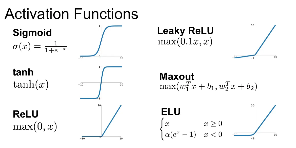
The binary step function is great for binary output. But, we want our neural network to be able to learn from its error. This can not be possible given the fact that activation functions should be continuous and differentiable to be able to do gradient descent, and the step function is not. down here are other most popular alternative activation functions.
Keep in mind that in older to apply gradient descent(reducing network error ), error function should be differentiable and continous.
Sigmoid Function
The sigmoid function is among the most common activation functions. as you see in the image above it is between 0 and 1, which makes sense for probabilistic models given the fact that probability exists between 0 and 1.

It simply mimics the activation behavior of a step function while being differentiable. It also has a very simple derivative that that can be calculated from the sigmoid function itself.
Conceptually, the sigmoid function makes decisions. When given weighted features from some data, it indicates whether or not the features contribute to classification. In that way, a sigmoid activation works well following a linear transformation. As it stands right now with random weights and bias, the sigmoid node’s output is also random. The process of learning through backpropagation and gradient descent modifies the weights and bias such that activation of the sigmoid node begins to match expected outputs.
here is sigmoid in programmer's language
class Sigmoid(Node):
    """
    Represents a node that performs the sigmoid activation function.
    """
    def __init__(self, node):
        # The base class constructor.
        Node.__init__(self, [node])

    def _sigmoid(self, x):
        """
        This method is separate from `forward` because it
        will be used with `backward` as well.
        `x`: A numpy array-like object.
        """
        return 1. / (1. + np.exp(-x))

    def forward(self):
        """
        Perform the sigmoid function and set the value.
        """
        input_value = self.inbound_nodes[0].value
        self.value = self._sigmoid(input_value)
Yeah like that our network now is continuous and differentiable.
Eventually, We will have to figure out how to measure our network accuracy. Let's say for example in the picture below that our neural network is trying to separate red dots from blue ones. given the fact that there are misclassified points there, thus we can measure how far we are to better classify every point right by calculating the summation Errors we made against each and every point.
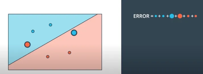
You might have noticed that the bigger the point the bigger the error(misclassification) in the image above. this perfectly mimics the perceptron trick whereby each and every point will have to communicate what is best for it to be classified well. Let’s break down some ways our points communicate to an entire network what they want, and it's a matter of the network to take actions that maximize the profit of each and every point on average.
Error Functions
There are a couple of techniques for defining the accuracy of a neural network. Some call then loss or cost.
There are many Types of Error Functions but in our case, we will use mean square error. The image below shows some maths of our error function.
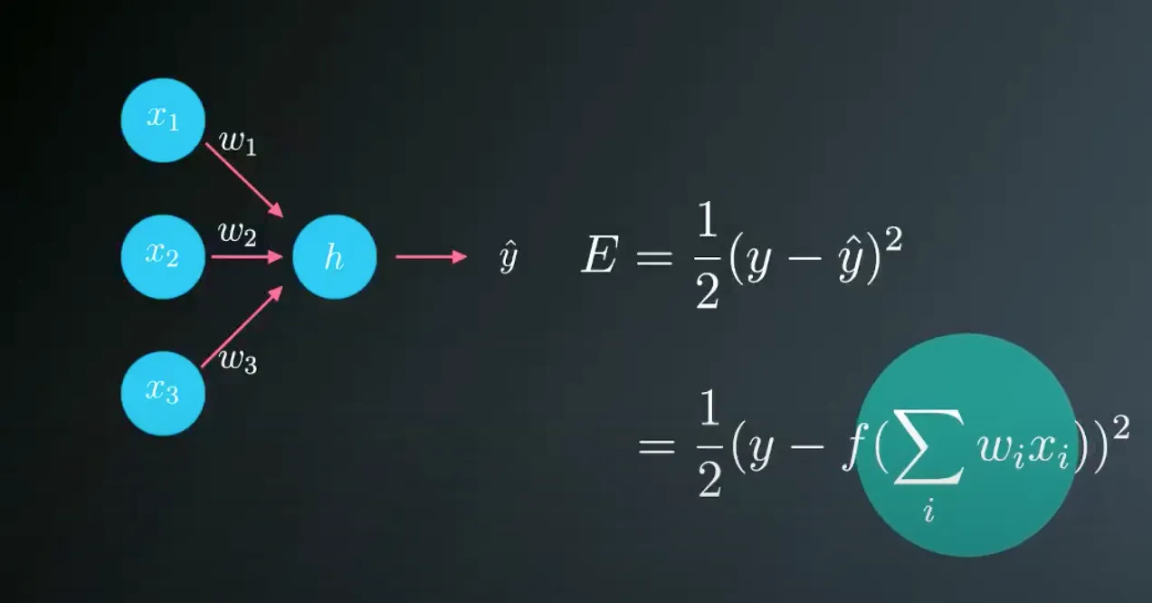
As you might have noticed, the above error function is the mean of the squares of the differences between the predictions and the labels. which will help us to measure our model accuracy.
we square the error becouse it helps penalize outliers more than small errors, and it also makes the maths simple later since we don’t want negative values if we happen to have positive errors
It is obvious the error is the function of the weights, and we will be using them to tune our network to make good predictions.
here is the code implementation!
class MSE(Node):
    def __init__(self, y, a):
        """
        The mean squared error cost function.
        Should be used as the last node for a network.
        """
        # Call the base class' constructor.
        Node.__init__(self, [y, a])

    def forward(self):
        """
        Calculates the mean squared error.
        """
        # NOTE: We reshape these to avoid possible matrix/vector broadcast
        # errors.
        #
        # For example, if we subtract an array of shape (3,) from an array of shape
        # (3,1) we get an array of shape(3,3) as the result when we want
        # an array of shape (3,1) instead.
        #
        # Making both arrays (3,1) insures the result is (3,1) and does
        # an elementwise subtraction as expected.
        y = self.inbound_nodes[0].value.reshape(-1, 1)
        a = self.inbound_nodes[1].value.reshape(-1, 1)
        m = self.inbound_nodes[0].value.shape[0]

        diff = y - a
        self.value = np.mean(diff**2)
Note the order of y and a doesn't actually matter, we could switch them around (a - y) and get the same value after being squared.
after getting errors of course we will have to find a way to decrease our errors for the network to better predict values.
Gradient Descent
Our goal is to make our network output as close as possible to the target values by minimizing the cost or its error. You can envision the cost or error as a mountain and we want descent to the bottom.
Since we know how wrong the predictions are, Now it’s time to descent from the error mountain. We need to update our weight to make predictions as close as possible to the real values. and the process is called Gradient Descent.
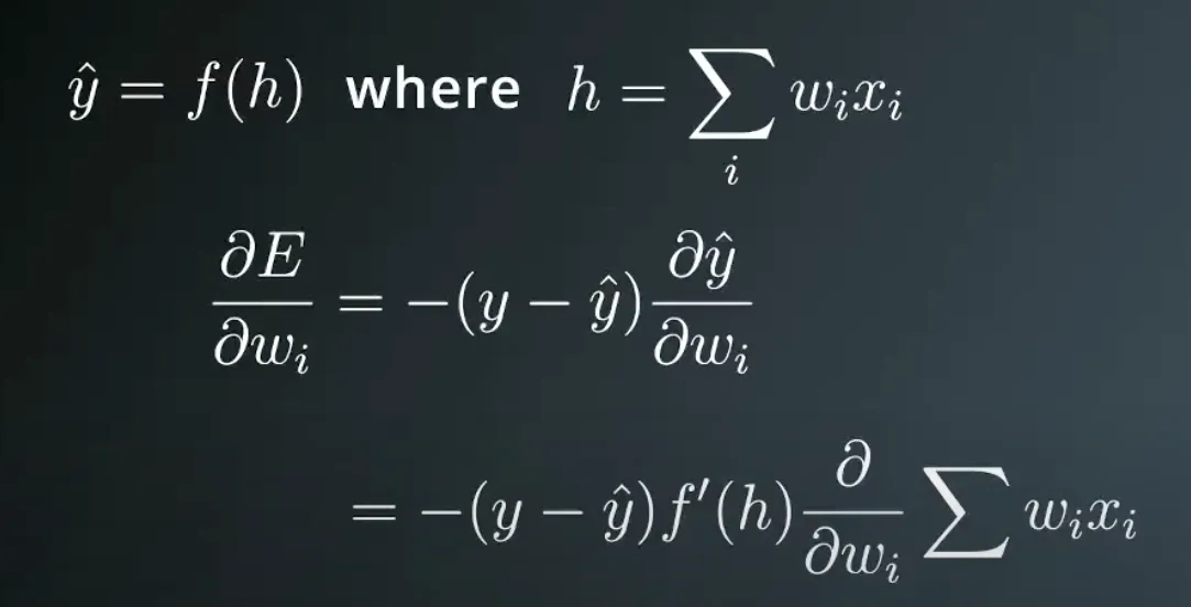
Our goal is to calculate the gradient of Error(E), at a point x = (x1,…, xn), given by the partial derivatives. We will simply calculate the derivative of the error that each point produces. We have seen the formula of the sum of the Error function in the above sections in case you need to revise.
In order to calculate the derivative of this error with respect to the weights, we’ll first calculate The predictions derivative with respect to weighs. below is the formula.
And now we can calculate the derivative of the error E at a point x.
to summarize this, the formula actually tells us that the Gradient of E with respect to point X is ∇E=−(y−y^)(x1,…,xn,1).
The gradient is the difference between the label and the prediction, times the coordinates of the point!
This means the closer the label to the prediction the smaller the gradiemt, Vise versa.
Since the gradient is a vector of numbers. Each number represents the amount by which we should adjust a corresponding weight or bias in the neural network. Adjusting all of the weights and biases by the gradient values reduces the cost (or error) of the network.
Now let’s take a walk to the bottom of the Error mountain.
Here the confusing part is how do we know which way is downhill. Well, the good news is, our gradient descent provides this exact information. it gives us the direction of the steepest descent, which is what we want.
Gradient Descent Step
Now we know the direction. The next thing to consider is how fast. or how long is our one step to the given direction? This is known as the learning rate, which is a value that determines how quickly or slowly the neural network learns.
You're probably thinking of big learning late, to make networks learn fast. But, Be careful! If the value is too large we could overshoot the target and eventually diverge from it. Yikes!

Convergence. This is the ideal behavior.
Divergence. This can happen when the learning rate is too large.
So what is a good learning rate, then?
This is more of a guessing game than anything else but empirically values in the range 0.1 to 0.0001 work well. The range 0.001 to 0.0001 is popular, as 0.1 and 0.01 are sometimes too large.
so basically gradient descent formula is x = x - learning_rate * gradient_of_x
Here’s the formula :
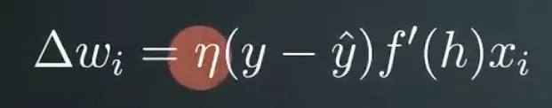
x is a parameter used by the neural network (i.e. a single weight or bias) and n is a learning rate.
let's apply this in codes :
def gradient_descent(x, gradx, learning_rate):
    """
    Performs a gradient descent update.
    """
    x = x - learning_rate * gradx
    # Return the new value for x
    return x
“you can’t connect the dots looking forward, you can only connect them looking backward”
Steve Job.
Backward Propagation
Wonder how will our network learn then. well by varying the weights, our NN can vary the amount of influence any given input has on the output now. It can also modify the weights and biases to improve the network’s output accuracy. and that’s backpropagation.
for us to do backpropagation we need a proper way to measure our network accuracy.
As you can see in this animation above after backpropagation our network adjusts in a way that produces accurate output than before.
Working through an example
Let’s walk through the steps of calculating the weight updates for a simple two-layer network. Suppose there are two input values, one hidden unit, and one output unit, with sigmoid activations on the hidden and output units.
Assume our target value y=1. We’ll start with the forward pass, first calculating the input to the hidden unit which is
h=∑i wi xi = 0.1×0.4−0.2×0.3=−0.02.
and the output of the hidden unit by simply applying the sigmoid function.
a=f(h)=sigmoid(−0.02)=0.495.
Using this as the input to the output unit, the output of the network is
y^=f(W⋅a)=sigmoid(0.1×0.495)=0.512.
With the network output, we can start the backward pass to calculate the weight updates for both layers. remember our sigmoid nice derivative.
the error term for the output unit is
δo=(y−y^)f′(W⋅a)=(1−0.512)×0.512×(1−0.512)=0.122
and error term for our hidden is
δh=Wδof′(h)=0.1×0.122×0.495×(1−0.495)=0.003
Now that we can calculate errors with respect to a given point, we can calculate the gradient descent steps. The hidden to output weight step is the learning rate, times the output unit error, times the hidden unit activation value.
so the gradient descent step calculation is as simple as this.
ΔW=ηδoa=0.5×0.122×0.495=0.0302
and the gradient descent step for the input node
Δwi=ηδhxi=(0.5×0.003×0.1,0.5×0.003×0.3)=(0.00015,0.00045)
so like this we backpropagate through the network and update the weight :
here is the complete code implementation so far
import numpy as np

class Node:
    """
    Base class for nodes in the network.

    Arguments:

        `inbound_nodes`: A list of nodes with edges into this node.
    """
    def __init__(self, inbound_nodes=[]):
        """
        Node's constructor (runs when the object is instantiated). Sets
        properties that all nodes need.
        """
        # A list of nodes with edges into this node.
        self.inbound_nodes = inbound_nodes
        # The eventual value of this node. Set by running
        # the forward() method.
        self.value = None
        # A list of nodes that this node outputs to.
        self.outbound_nodes = []
        # New property! Keys are the inputs to this node and
        # their values are the partials of this node with
        # respect to that input.
        self.gradients = {}
        # Sets this node as an outbound node for all of
        # this node's inputs.
        for node in inbound_nodes:
            node.outbound_nodes.append(self)

    def forward(self):
        """
        Every node that uses this class as a base class will
        need to define its own `forward` method.
        """
        raise NotImplementedError

    def backward(self):
        """
        Every node that uses this class as a base class will
        need to define its own `backward` method.
        """
        raise NotImplementedError


class Input(Node):
    """
    A generic input into the network.
    """
    def __init__(self):
        # The base class constructor has to run to set all
        # the properties here.
        #
        # The most important property on an Input is value.
        # self.value is set during `topological_sort` later.
        Node.__init__(self)

    def forward(self):
        # Do nothing because nothing is calculated.
        pass

    def backward(self):
        # An Input node has no inputs so the gradient (derivative)
        # is zero.
        # The key, `self`, is reference to this object.
        self.gradients = {self: 0}
        # Weights and bias may be inputs, so you need to sum
        # the gradient from output gradients.
        for n in self.outbound_nodes:
            self.gradients[self] += n.gradients[self]

class Linear(Node):
    """
    Represents a node that performs a linear transform.
    """
    def __init__(self, X, W, b):
        # The base class (Node) constructor. Weights and bias
        # are treated like inbound nodes.
        Node.__init__(self, [X, W, b])

    def forward(self):
        """
        Performs the math behind a linear transform.
        """
        X = self.inbound_nodes[0].value
        W = self.inbound_nodes[1].value
        b = self.inbound_nodes[2].value
        self.value = np.dot(X, W) + b

    def backward(self):
        """
        Calculates the gradient based on the output values.
        """
        # Initialize a partial for each of the inbound_nodes.
        self.gradients = {n: np.zeros_like(n.value) for n in self.inbound_nodes}
        # Cycle through the outputs. The gradient will change depending
        # on each output, so the gradients are summed over all outputs.
        for n in self.outbound_nodes:
            # Get the partial of the cost with respect to this node.
            grad_cost = n.gradients[self]
            # Set the partial of the loss with respect to this node's inputs.
            self.gradients[self.inbound_nodes[0]] += np.dot(grad_cost, self.inbound_nodes[1].value.T)
            # Set the partial of the loss with respect to this node's weights.
            self.gradients[self.inbound_nodes[1]] += np.dot(self.inbound_nodes[0].value.T, grad_cost)
            # Set the partial of the loss with respect to this node's bias.
            self.gradients[self.inbound_nodes[2]] += np.sum(grad_cost, axis=0, keepdims=False)


class Sigmoid(Node):
    """
    Represents a node that performs the sigmoid activation function.
    """
    def __init__(self, node):
        # The base class constructor.
        Node.__init__(self, [node])

    def _sigmoid(self, x):
        """
        This method is separate from `forward` because it
        will be used with `backward` as well.

        `x`: A numpy array-like object.
        """
        return 1. / (1. + np.exp(-x))

    def forward(self):
        """
        Perform the sigmoid function and set the value.
        """
        input_value = self.inbound_nodes[0].value
        self.value = self._sigmoid(input_value)

    def backward(self):
        """
        Calculates the gradient using the derivative of
        the sigmoid function.
        """
        # Initialize the gradients to 0.
        self.gradients = {n: np.zeros_like(n.value) for n in self.inbound_nodes}
        # Sum the partial with respect to the input over all the outputs.
        for n in self.outbound_nodes:
            grad_cost = n.gradients[self]
            sigmoid = self.value
            self.gradients[self.inbound_nodes[0]] += sigmoid * (1 - sigmoid) * grad_cost


class MSE(Node):
    def __init__(self, y, a):
        """
        The mean squared error cost function.
        Should be used as the last node for a network.
        """
        # Call the base class' constructor.
        Node.__init__(self, [y, a])

    def forward(self):
        """
        Calculates the mean squared error.
        """
        # NOTE: We reshape these to avoid possible matrix/vector broadcast
        # errors.
        #
        # For example, if we subtract an array of shape (3,) from an array of shape
        # (3,1) we get an array of shape(3,3) as the result when we want
        # an array of shape (3,1) instead.
        #
        # Making both arrays (3,1) insures the result is (3,1) and does
        # an elementwise subtraction as expected.
        y = self.inbound_nodes[0].value.reshape(-1, 1)
        a = self.inbound_nodes[1].value.reshape(-1, 1)

        self.m = self.inbound_nodes[0].value.shape[0]
        # Save the computed output for backward.
        self.diff = y - a
        self.value = np.mean(self.diff**2)

    def backward(self):
        """
        Calculates the gradient of the cost.
        """
        self.gradients[self.inbound_nodes[0]] = (2 / self.m) * self.diff
        self.gradients[self.inbound_nodes[1]] = (-2 / self.m) * self.diff


def topological_sort(feed_dict):
    """
    Sort the nodes in topological order using Kahn's Algorithm.

    `feed_dict`: A dictionary where the key is a `Input` Node and the value is the respective value feed to that Node.

    Returns a list of sorted nodes.
    """

    input_nodes = [n for n in feed_dict.keys()]

    G = {}
    nodes = [n for n in input_nodes]
    while len(nodes) > 0:
        n = nodes.pop(0)
        if n not in G:
            G[n] = {'in': set(), 'out': set()}
        for m in n.outbound_nodes:
            if m not in G:
                G[m] = {'in': set(), 'out': set()}
            G[n]['out'].add(m)
            G[m]['in'].add(n)
            nodes.append(m)

    L = []
    S = set(input_nodes)
    while len(S) > 0:
        n = S.pop()

        if isinstance(n, Input):
            n.value = feed_dict[n]

        L.append(n)
        for m in n.outbound_nodes:
            G[n]['out'].remove(m)
            G[m]['in'].remove(n)
            # if no other incoming edges add to S
            if len(G[m]['in']) == 0:
                S.add(m)
    return L


def forward_and_backward(graph):
    """
    Performs a forward pass and a backward pass through a list of sorted Nodes.

    Arguments:

        `graph`: The result of calling `topological_sort`.
    """
    # Forward pass
    for n in graph:
        n.forward()

    # Backward pass
    # see: https://docs.python.org/2.3/whatsnew/section-slices.html
    for n in graph[::-1]:
        n.backward()


def sgd_update(trainables, learning_rate=1e-2):
    """
    Updates the value of each trainable with SGD.

    Arguments:

        `trainables`: A list of `Input` Nodes representing weights/biases.
        `learning_rate`: The learning rate.
    """
    # Performs SGD
    #
    # Loop over the trainables
    for t in trainables:
        # Change the trainable's value by subtracting the learning rate
        # multiplied by the partial of the cost with respect to this
        # trainable.
        partial = t.gradients[t]
        t.value -= learning_rate * partial
Now Our network has the capability to learn and make smart decisions for itself. It’s that time to investigate ourselves haha. Let's try to diagnose breast cancer from online datasets.
# from sklearn.datasets import load_boston
from sklearn.utils import shuffle, resample
from sklearn.datasets import load_breast_cancer


# Load data
# data = load_boston()
data = load_breast_cancer()
X_ = data['data']
y_ = data['target']

# Normalize data
X_ = (X_ - np.mean(X_, axis=0)) / np.std(X_, axis=0)

n_features = X_.shape[1]
n_hidden = 100
W1_ = np.random.randn(n_features, n_hidden)
b1_ = np.zeros(n_hidden)
W2_ = np.random.randn(n_hidden, 1)
b2_ = np.zeros(1)

# Neural network
X, y = Input(), Input()
W1, b1 = Input(), Input()
W2, b2 = Input(), Input()

l1 = Linear(X, W1, b1)
s1 = Sigmoid(l1)
l2 = Linear(s1, W2, b2)
cost = MSE(y, l2)

feed_dict = {
    X: X_,
    y: y_,
    W1: W1_,
    b1: b1_,
    W2: W2_,
    b2: b2_
}

epochs = 1000
# Total number of examples
m = X_.shape[0]
batch_size = 11
steps_per_epoch = m // batch_size

graph = topological_sort(feed_dict)
trainables = [W1, b1, W2, b2]

print("Total number of examples = {}".format(m))

# Step 4
for i in range(epochs):
    loss = 0
    for j in range(steps_per_epoch):
        # Step 1
        # Randomly sample a batch of examples
        X_batch, y_batch = resample(X_, y_, n_samples=batch_size)

        # Reset value of X and y Inputs
        X.value = X_batch
        y.value = y_batch

        # Step 2
        forward_and_backward(graph)

        # Step 3
        sgd_update(trainables)

        loss += graph[-1].value

    print("Epoch: {}, Loss: {:.3f}".format(i+1, loss/steps_per_epoch))
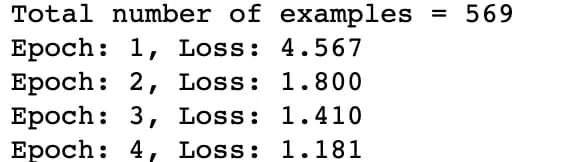
as you can see our learning loss has diminished from 4.567 up to 0.069 on the 100th epoch.
Yay! our network is able to learn and become wise. Let’s test it in the image dataset.
Lets's use our algorithm to visually diagnose melanoma, the deadliest form of skin cancer.
To be continued….
Recommended Improvements Local minima, Breakpoint